|
|
In wireless networks [102, 45], computers are connected and communicate with each other not by a visible medium, but by emissions of electromagnetic energy in the air.
The most widely used transmission support is radio waves. Wireless transmissions utilize the microwave spectre: the available frequencies are situated around the 2.4 GHz ISM (Industrial, Scientific and Medical) band for a bandwidth of about 83 MHz, and around the 5 GHz U-NII (Unlicensed-National Information Infrastructure) band for a bandwidth of about 300 MHz divided into two parts. The exact frequency allocations are set by laws in the different countries; the same laws also regulate the maximum allotted transmission power and location (indoor, outdoor). Such a wireless radio network has a range of about 10–100 meters to 10 Km per machine, depending on the emission power, the data rate, the frequency, and the type of antenna used. Many different models of antenna can be employed: omnis (omnidirectional antennas), sector antennas (directional antennas), yagis, parabolic dishes, or waveguides (cantennas).
The other type of transmission support is the infrared. Infrared rays cannot penetrate opaque materials and have a smaller range of about 10 meters. For these reasons, infrared technology is mostly used for small devices in WPANs (Wireless Personal Area Networks), for instance to connect a PDA to a laptop inside a room.
There are presently three main standards for wireless networks: the IEEE 802.11 family, HiperLAN, and Bluetooth.
IEEE 802.11 [108] is a standard issued by the IEEE (Institute of Electrical and Electronics Engineers). From the point of view of the physical layer, it defines three non-interoperable techniques: IEEE 802.11 FHSS (Frequency Hopping Spread Spectrum) and IEEE 802.11 DSSS (Direct Sequence Spread Spectrum), which use both the radio medium at 2.4 GHz, and IEEE 802.11 IR (InfraRed). The achieved data rate is 1–2 Mbps. This specification has given birth to a family of other standards:
Another standard currently under development, IEEE 802.16 [75] (marketed as WiMAX), is designed for WMANs (Wireless Metropolitan Area Networks) and therefore to overcome the range limitations of IEEE 802.11. It operates on frequencies from 10 to 66 GHz, and should ensure network coverage for several square Km. From the IEEE 802.16 standard derives IEEE 802.16a, that operates on the 2-11 GHz band and should solve the line-of-sight problems deriving from using the 10-66 GHz band.
The crucial point in channel access techniques for wireless networks is that it is not possible to transmit and to sense the carrier for packet collisions at the same time. Therefore there is no way to implement a CSMA/CD (Carrier Sense Multiple Access / Collision Detection) protocol such as in the wired Ethernet.
IEEE 802.11 uses a channel access technique of type CSMA/CA, which is meant to perform Collision Avoidance (or at least to try to). The CSMA/CA protocol states that a node, upon sensing that the channel is busy, must wait for an interframe spacing before attempting to transmit, then choose a random delay depending on the Contention Window.
The reception of a packet is acknowledged by the receiver to the sender. If the sender does not receive the acknowledgement packet, it waits for a delay according to the binary exponential backoff algorithm, which states that the Contention Window size is doubled at each failed try.
Unicast data packets are sent using a more reliable mechanism. The source transmits a RTS (Request To Send) packet for the destination, which replies with a CTS (Clear To Send) packet upon reception. If the source correctly receives the CTS, it sends the data packet.
HiperLAN (High Performance Radio LAN) is a standard issued by the ETSI (European Telecommunications Standard Institute), and a competitor of IEEE 802.11. It defines two kinds of networks:
A related standard is HiperMAN, rival of IEEE 802.16 and aimed at providing metropolitan area coverage. It operates in the 2–11 GHz band.
Bluetooth1 is a standard designed by a consortium of private companies such as Agere, Ericsson, IBM, Intel, Microsoft, Motorola, Nokia and Toshiba. Bluetooth operates in the 2.4 GHz band using FHSS and has a short range of action of about 10 meters. For such characteristics and its low cost, Bluetooth is fit for small WPANs and is also employed to connect peripherals such as keyboards, printers, or mobile phone headsets. Bluetooth radio technology works in a master-slave fashion, and each device can operate as master or as slave. Communications are organized in small networks called piconets, each piconet being composed of a master and 1–7 active slaves. Multiple piconets can overlap to form a scatternet.
A wireless network can be structured to function in either BSS (Basic Service Set) or IBSS (Independent Basic Service Set) mode. The two modes affect the topology and the mobility capabilities of the machines (nodes) that compose the network.
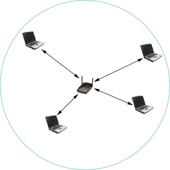
In BSS mode, also called infrastructure mode, a number of mobile nodes are wirelessly connected to a non-mobile Access Point (AP), as in Figure 1.1. Nodes communicate via the AP, which may also provide connectivity with an external wired network e.g. the Internet. Several BSS networks may be joined to form an ESS (Extended Service Set).
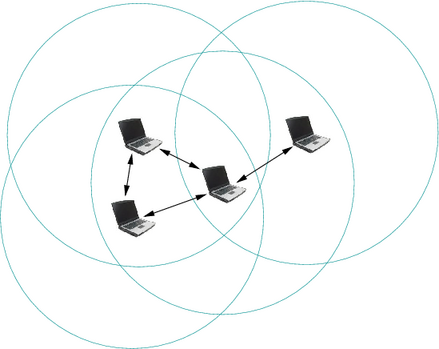
The IBSS mode, also called peer to peer or ad hoc mode, allows nodes to communicate directly (point-to-point) without the need for an AP, as in Figure 1.2. There is no fixed infrastructure. Nodes need to be in range with each other in order to communicate.
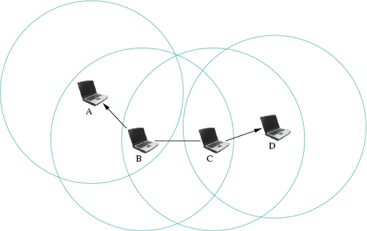
An ad hoc network, or MANET (Mobile Ad hoc NETwork), is a network composed only of nodes, with no Access Point. Messages are exchanged and relayed between nodes. In fact, an ad hoc network has the capability of making communications possible even between two nodes that are not in direct range with each other: packets to be exchanged between these two nodes are forwarded by intermediate nodes, using a routing algorithm.2 Hence, a MANET may spread over a larger distance, provided that its ends are interconnected by a chain of links between nodes (also called routers in this architecture). In the ad hoc network shown in Figure 1.3, node A can communicate with node D via nodes B and C, and vice versa.
A sensor network is a special class of ad hoc network, composed of devices equipped with sensors to monitor temperature, sound, or any other environmental condition. These devices are usually deployed in large number and have limited resources in terms of battery energy, bandwidth, memory, and computational power.
A wireless network offers important advantages with respect to its wired homologue:
On the other hand, there are some drawbacks that need to be pondered:
In ad hoc networks, to ensure the delivery of a packet from sender to destination, each node must run a routing protocol and maintain its routing tables in memory.
Routing protocols can be classified into the following categories: reactive, proactive, and hybrid. There exists nowadays almost one hundred routing protocols, many standardized by the IETF (Internet Engineering Task Force) and others still at the stage of Internet-Draft. This section gives, for each category, an overview of the most important ones.
Under a reactive (also called on-demand) protocol, topology data is given only when needed. Whenever a node wants to know the route to a destination node, it floods the network with a route request message. This gives a reduced average control traffic, with bursts of messages when packets need being routed, and an additional delay due to the fact that the route is not immediately available.
In opposition, proactive (also called periodic or table driven) protocols are characterized by periodic exchange of topology control messages. Nodes periodically update their routing tables. Therefore, control traffic is more dense but constant, and routes are instantly available.
Hybrid protocols have both the reactive and proactive nature. Usually, the network is divided into regions, and a node employs a proactive protocol for routing inside its near neighborhood’s region and a reactive protocol for routing outside this region.
The Optimized Link State Routing (OLSR) protocol [31, 79, 29] is a proactive link state routing protocol for ad hoc networks.
The core optimization of OLSR is the flooding mechanism for distributing link state information, which is broadcast in the network by selected nodes called Multipoint Relays (MPR). As a further optimization, only partial link state is diffused in the network. OLSR provides optimal routes (in terms of number of hops) and is particularly suitable for large and dense networks.
Specifications of the protocol were first described in an Internet-Draft in February 2000, and were finalized in RFC 3626 [31] in October 2003; there is also a draft for the version 2 of the protocol [27]. Several implementations exist at this day: OOLSR (the original, object-oriented implementation of OLSR by INRIA HIPERCOM), nlrolsrd (by the U.S. Naval Research Laboratory), OLSR_Niigata (by Niigata University), Qolyester (a Quality-of-Service enhanced version by LRI), OLSR11win (by the GRC, Universitat Politècnica de València), the olsr.org OLSR daemon (by UniK, University of Oslo), H-OLSR (by Hitachi, Ltd.), and CRC OLSR (by the Communication Research Centre in Canada). A multicast extension [95] has been proposed and is the object of an Internet-Draft (MOLSR) [80].
OLSR control messages are communicated using a transport protocol defined by a general packet format, given in Figure 1.5. Each packet encapsulates several control messages into one transmission.
Control traffic in OLSR is exchanged through two different types of messages: HELLO and TC (Topology Control) messages. HELLO messages, shown in Figure 1.6, are exchanged periodically among neighbor nodes, in order to detect links to neighbors and to signal MPR selection. TC messages, shown in Figure 1.7, are periodically flooded to the entire network, in order to diffuse link state information to all nodes.
The other OLSR control messages are MID (Multiple Interface Declaration) and HNA (Host and Network Association). MID and HNA messages are emitted only by nodes that have multiple interfaces. To avoid collisions, the OLSR protocol adds an amount of jitter to the interval at which all control messages are generated.
While messages may potentially be broadcast to the entire network, packets are transmitted only between neighbor nodes. The unit of information subject to being forwarded is a “message”. An individual OLSR control message can be uniquely identified by its Originator Address and Message Sequence Number (MSN), both from the message header. The Originator Address field specifies the originator of a message, and does not change as the message is relayed around the network; the address contained in this field is different (except at the first hop, when the message is created) from the IP header source address, which is changed at each hop to the address of the retransmitting node.
A node may receive the same message several times. Therefore, to avoid processing and sending multiple times the same message, a node records information about each received message. This information is stored in a tuple consisting of the message’s originator address, the MSN, a boolean value indicating whether the message has already been retransmitted, the list of interfaces on which the message has been received, and the tuple’s expiration time. All tuples are maintained in the Duplicate Set (also known as Duplicate Table) of the node.
The common packet format allows individual messages to be piggybacked and transmitted together in one emission, if allowed by the MTU size. Therefore different kind of control messages can be emitted together, although processed and forwarded differently in each node; e.g. HELLO messages are not forwarded while all other control messages are.
OLSR does not handle unicast communications: a message from a node is either transmitted to all its neighbors or to all nodes in the network.
|
| |||||||||||||||||||||||||||||||||||||
Upon receiving a HELLO message, a node examines the lists of addresses. If its own address is included in the addresses encoded in the HELLO message, bidirectional communication is possible (symmetrical link) between the originator and the recipient of the HELLO message, i.e. the node itself.
In addition to information about neighbor nodes, periodic exchange of HELLO messages allows each node to maintain information describing the links between neighbor nodes and nodes which are two hops away. This information is recorded in a nodes 2-hop neighbor set and is utilized for MPR optimization.
HELLO messages are exchanged periodically between neighbor nodes only, and are not forwarded further.
|
The TC message bears an ANSN field which contains the Advertised Neighbor Sequence Number. This number is associated with the node’s advertised neighbor set, and is incremented each time the node detects a change in this set.
|
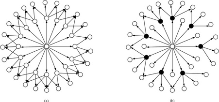
The OLSR backbone for message flooding is composed of Multipoint Relays. Each node must select MPRs from among its symmetric neighbor nodes such that a message emitted by a node and repeated by the MPR nodes will be received by all nodes two hops away. In fact, in order to achieve a network-wide broadcast, a broadcast transmission needs only be repeated by just a subset of the neighbors: this subset is the MPR set of the node. Hence only MPR nodes relay TC, MID, and HNA messages.
Figure 1.8 shows the node in the center, with neighbors and 2-hop neighbors, broadcasting a message. In (a) all nodes retransmit the broadcast, while in (b) only the MPRs of the central node retransmit the broadcast.
The MPR set of a node is computed heuristically [129]. MPR selection is performed based on the 2-hop neighbor set received through the exchange of HELLO messages, and is signaled through the same mechanism. Each node maintains an MPR selector set, describing the set of nodes that have selected it as MPR.
The standard OLSR specification document does not take account of security measures. It enumerates possible vulnerabilities to which OLSR is subject. These vulnerabilities include breach of confidentiality, breach of integrity, non-relaying, replay, and interaction with an insecure external routing domain.
We give in Chapter 2 a brief overview on system security, and in Chapter 3 a
detailed description of the attacks against OLSR and against the routing
protocols in general. A mechanism designed to secure the OLSR protocol is
presented in Chapter 5.